We are certainly living longer than ever before. But within that statement lie a number of interesting stories neatly summarised by the Office of National Statistics (ONS) report on average life span in England and Wales, which came out around a year ago.

The first graph below has been constructed by first devising a rather artificial thing called a life table. This starts with 100,000 people at birth for each year and then, based on the probability of dying in the first year of life, works out how many are expected to survive to age 1. Of those, the probability of dying in the second year is applied to the number at year 1 in the table to work out the expected number of deaths during the second year. These are then deducted from the year 1 entry to arrive at the year 2 entry. And so on. Skip the next paragraph if that explanation is enough for you.

So, for example, taking the data from the England & Wales interim life tables 2009-11, we have 100,000 males at age 0, 99,508.2 at age 1 and 99,475.2 at age 2. This is because the probability of death for males in the first year of life over the 3 year period 2009 to 2011 was 0.004918, so 100,000 x 0.004918 = 491.8 expected deaths and 100,000 – 491.8 = 99,508.2 expected to be left in this imaginary population to celebrate their first birthdays. The probability of death in the second year of life was 0.000331 (notice this is much smaller, we will return to the significance of this later) so that the number of boys getting to blow two candles out on a cake is expected to be 99,508.2 – (0.000331 x 99,508.2) = 99,475.2. This table is nothing like real life of course, as we all move through time as we get older, so that our chance of death at age 20, say, would not be the same as the chance of a 20 year old dying 20 years earlier. However such a table does allow us to illustrate the patterns of deaths in any given year, and then compare these with other years.

The three measures used are based on the three averages you learned at school: the mean, median and mode.

The life expectancy at birth is a form of mean. The probability of reaching each age can be calculated by looking how many people you have at that age in your imaginary life table and dividing that number by the 100,000 you started with. Then each of these probabilities is multiplied by the age reached and then the probability of dying in that year (strictly the ONS life tables are constructed by taking the average probability for each year as the mid point between the start of the year and end of year probability, with a further adjustment in the first year when the probability of death is very much concentrated in the first 4 weeks). This can be shown to be same as all the entries (from year 1, year 2, year 3, etc) in the life table added up and divided by the 100,000 you started with.

The median is the age at which we expect half the population to have died. The mode is the age at which we see the highest number of deaths. The mode here has been adjusted in two further ways: the deaths below age 10 have been removed (otherwise it would have been 0 in a number of years and it is the old age mortality we are looking to compare) and it has also been smoothed to take out year on year fluctuations caused by wars and flu pandemics (again this would lead to modes in the 20s and 30s in some years, which are not the ages we are focused on).

life expectancy

There are many features to this graph, as set out in the ONS paper. The closing down of the gap between the mode on the one hand, and the median and life expectancy at birth on the other, is especially striking. This was mainly due to the massive improvement in survival rates in the first year in birth in particular. It also demonstrates that, contrary to what we might have believed about Victorian England, plenty of people were living into their 70s in the 1840s.

However I want to focus on the race to live longer between men and women because, armed with these three numbers (or six as we are looking at men and women separately) for each year, we can see that men and women have had a rather different journey since 1841.

As we can see the experience was fairly similar in the 1840s, although even then women lived 2 or 3 years longer on the mean and median measures than men. The modal age at death was more variable due to the relatively small numbers at advanced ages in the early years, but was between 25 and 30 years in excess of the median and life expectancy at birth due to the relatively high level of infant and child deaths at the time. The median and life expectancy then steadily advanced on the mode (interrupted by two downward spikes: in the mid 1840s a combined assault of typhus, flu and cholera, and a much larger one in 1919 from the flu pandemic).

In 1951, the female median age at death moved above the male modal age for the first time, marking the start of a 20 year period where life expectancy increases on all measures for women exceeded those of men. While the commonest age of death for men stayed in the mid 70s over this period, that for women increased from 79.5 to 82.5, leading to a peak difference in commonest age of death between men and women of 8.5 years in 1971. A graph of the differences in all three averages is shown below.

Differences life expectancies

Since 1971 the tide has turned, with all six lines steadily, if very gradually, converging. In 2010 the male modal age at death finally crossed back over the female life expectancy at birth, and all three differences fell below 4 years for the first time since 1926. As the Longevity Science Advisory Panel’s second report points out, the average differences between life expectancy by gender at birth of 4.15 between 2005 and 2009 represent, in terms of the percentage of female life expectancy (5.1%), a return to the levels seen at the start of the journey in 1841. In 2010 this percentage fell to 4.7%. It has only fallen below that level four times since 1841, and not since 1857.

So we may be entering a new phase in the expected longevity differences between men and women. And, as the history shows us, those differences can change with surprising speed.

The latest figures (January 2014) from the European Central Bank (ECB) statistics pocket book have just been issued, providing comparisons between European Union (EU) countries, both in the Eurozone and outside it, on a range of measures. And some of these comparisons are not quite what I expected to see.

For instance, perhaps surprisingly in view of the current hysteria in the UK about economic migrants from Bulgaria and Romania, we find that unemployment was lower in Romania (7.3%) than it is in the UK (7.4%) for the latest month (September 2013) for which data on both was available (it’s the UK’s that is missing for October and November for reasons unknown).

I have graphed a selection of the data below, Euro countries are to the left:

ECB country data labelled

First to note, which may also surprise some, is that private sector debt in the UK is not particularly big in EU terms: Denmark and Sweden both have considerably higher private sector debt as a percentage of GDP than the UK, as do 7 countries in the Eurozone with Ireland and Luxembourg heading the list.

Government expenditure as a percentage of GDP is the most evenly distributed of all the measures. I have graphed the 2012 data, as the Q2 2013 data omitted France and Germany. The range across all countries is between 36.1% (Lithuania) and 59.5% (Denmark), with the UK’s 47.9% only a little below the Eurozone average of 49.9%. This suggests to me, for all of the political rhetoric we hear, that it is not the total spend which tends to alter much but the distribution of it. Certainly in the UK, there appears to have been a focus on a relatively small section of the welfare budget to make the savings from.

Government debt is much higher as a proportion of GDP in the Eurozone than in the rest of the EU, with no one outside the Eurozone reaching the Eurozone average of 93.4% (although the UK comes closest at 89.8%). There are 5 countries in the Eurozone with debt above 100%: Belgium (perhaps surprisingly), Ireland, Greece, Italy and Portugal. Spain’s debt is actually below the Eurozone average at 92.3%.

Unemployment statistics are unsurprisingly dominated by Greece and Spain, whose unemployment rates are around 50% higher than the next country. Unemployment rates average 12.1% in the Eurozone and 10.9% for the EU as a whole, perhaps demonstrating the advantage of keeping control of your exchange rate during an economic downturn.

The population statistics remind me what an unusual decision it was for the UK to stay out of the Euro. All the other big countries (by which I mean those with populations over 45 million) are in the Eurozone, with the next biggest EU country outside the Euro being Poland at 38.5 million (with the prospect of their joining the Euro receding somewhat last year). Most of the richer countries are too, illustrated by a much higher proportion of GDP (see below) held in Eurozone countries than their relative populations would lead you to expect.

Finally we come to GDP. This looks very differently distributed according to whether you look at amounts in Euros, or per capita, or by capita adjusted for the purchasing power in each country. The first of these is dominated as expected by the big countries of Germany, Spain, France, Italy and the UK. However, the outstanding performer when looking at GDP per capita with or without the purchasing power adjustment is Luxembourg. Eurozone countries have a higher GDP per capita than those outside (€28,500 compared to €25,500, with the gap narrowing slightly when adjusted for purchasing power).

A final thing strikes me about these statistics. As has been pointed out elsewhere, Francois Hollande is having a hell of a time considering that France’s economic performance is not that bad. In fact it is incredibly average: its Government debt sits at 93.5% compared to the Eurozone average of 93.4% and its GDP per capita when adjusted for purchasing power is bang on the Eurozone average of €28,500. France are much more representative Euro members than Germany (remarkable when you consider that the Euro was once referred to as the Deutsche Mark with a few disreputable friends) and, if Hollande’s approval ratings are any indication, the French people seem to hate that.

I recently came across this post from 2009, showing how total returns companies achieved and the remuneration packages of their CEOs had no obvious relation between them. This kind of article, showing a correlation does not exist, is relatively unusual in my experience.

Far more common are articles like this one, by Eugenio Proto and Aldo Rustichini, purporting to show new evidence about the link between life satisfaction and GDP. Even if you accept whatever methodology they have used to derive their life satisfaction index (I don’t think we can get no satisfaction currently, see my previous blog), you have then to accept them defining a feature of the data entirely created by their regression analysis tool (the so-called “bliss point”) before going on to discuss what the implications of it might be.

The article’s references are stuffed with well-known economists’ papers and I am sure that one of its conclusions in particular, that increases in GDP beyond a certain point may not increase life satisfaction in developed countries, will lead to the research paper underlying the article to be widely cited as this is a politically contentious area. However this kind of thing is really nothing more than an economic Rorschach test: the meaning of the ink spots often depend on what you want to see.

But such studies are not often treated in this way. Why? Well what if one of the interpretations of the ink spots was backed up by some mathematics which could be run very quickly on any ink spot pattern by anyone with a computer? There is nothing biased about the mathematics, after all. This is what regression tools give us.

Regression is taught to sixth formers (I have taught it myself) as a way of finding best fit lines to data in a less subjective way than drawing lines by eye. The best fit straight line in a scatter graph is arrived at by looking at differences between the x and y coordinates of specific points and the average x and y values respectively. For y on x (ie assuming y is a function of x, you usually get a different gradient if you assume x is a function of y), the gradient of the line is the sum of each x value less its average times the corresponding y value less its average, all divided by the sum of the squares of the x values less their average. Or as a formula (the clumsiness of the preceding sentence is why we use formulae):

Correlation formula

Now let’s focus again on the graphs in the Proto and Rustichini article (the second graph has excluded Brussels and Paris, on the basis that they are both very rich and very miserable) and their regression-generated lines of best fit.

GDP life satisfaction

If we look long enough at these graphs we can almost persuade ourselves that the formula driven trend line (not a linear one this time) shown actually represents some feature of the data. But could you draw it yourself? And, if you did, would it look anything like the formula-generated one? If your answer is no to either of these questions, there is a possibility that the feature identified by Proto and Rustichini would be entirely absent from your trend line. The formula will always give you some sort of result. The trick is identifying when it is rubbish.

As an illustration of this, I constructed a graph where I was confident there was absolutely no correlation between the two things, and then set Excel’s regression tools to work on it.

Correlation obsession

As you can see, none of the options, starting with the linear regression we discussed earlier and getting more complicated, result in the kind of #DIV/0 and #N/A messages we get to see regularly elsewhere in Excel. By setting the polynomial option to a quintic, Excel is quite prepared to construct a best fit polynomial of order 5 (it has a fifth power in it – the purple wavy curve) to my array of dots. These lines and curves are merely the inevitable result of the mechanistic application of formulae that in this case have no meaning.

There may be nothing biased about the mathematics, but, as Bernard says In Yes Minister, when questioned by Jim Hacker about the impartiality of an enquiry: “Railway trains are impartial too, but if you lay down the lines for them that’s the way they go.”

Many economic research papers contain graphs which are similarly afflicted.

For those people who are not pensions geeks, let me start by explaining what the Pension Protection Fund (PPF) is. Brought in by the Pensions Act 2004 in response to several examples of people getting to retirement and finding little or no funds left in their defined benefit (DB) pension schemes to pay them benefits, it is a quasi autonomous non-governmental (allegedly) organisation (QUANGO) charged with accepting pension schemes who have lost their sponsors and don’t have enough money to buy at least PPF level benefits from an insurance company. It is, as the PPF themselves appear to have acknowledged with several references to the schemes not yet in their clutches as the “insured” in a talk I attended last week, a statutory insurance scheme for defined benefit occupational pension schemes, paid for by statutory levies on those insured. As a scheme actuary I have always been very glad that it exists.

The number of insured schemes has dwindled since it was named the 7800 index in 2007 (with not quite 7,800 members at the time) to the 6,300 left standing today. As you can imagine, the ever smaller number of schemes whose levies are keeping the PPF ship afloat are very nervous about how that cost is going to vary in the future. They have seen how volatile the funding of their own schemes is, and seemingly always in the worst case direction, and worry that, when their numbers get small enough, funding the variations in PPF deficits could become overwhelming. Particularly as the current Government says whenever it is asked (although no one completely believes it) they will never ever bail out the PPF.

So there has been keen interest in the PPF explanations of how those levies are going to change next year.

PPF levies are in two parts. The scheme-based levy, which is a flat rate levy based on the liability of a scheme, and the normally-much-bigger-as-it-has-to-raise-around-90%-of-the-total-and-some-schemes-don’t-pay-it-if-they-are-well-funded-enough risk-based levy. The risk-based levy depends on how well funded you are, how risky your investment strategy is and the risk your sponsor will become insolvent over the next 12 months.

It is this last one, the insolvency risk, which is about to change. Dun and Bradstreet have lost the contract to work out these insolvency probabilities after eight years in favour of Experian. However, unfortunately and for reasons not divulged, the PPF has struggled to finalise exactly what they want Experian to do.

The choices are fairly fundamental:

  • The model used. This will either be something called commercial Delphi (similar to the approach D&B currently use) or a more PPF-specific version which takes account of how different companies which run DB schemes are from companies which don’t. The PPF-specific version looks like it was originally the front runner but has taken longer to develop than expected.
  • The number of risk levels. Currently there are 10, ie there are 10 different probabilities of insolvency you can have based on the average risk of the bucket you have landed in. One possibility still being considered at this late stage is not grouping schemes at all and basing the probability on what falls out of the as yet to be announced risk model directly. This could result in considerable uncertainty about the eventual levy. Even currently, being in bucket 10 means a levy 22 times bigger than being in bucket 1.

So reason for nervousness amongst the 6,300 perhaps? The delay will mean that it won’t be known by 1 April (an appropriate date perhaps) when data starts to be collected for the first levies under the new system next year. Insolvency risk is supposed to be based on the average insolvency probability over the 12 months to the following March, but the PPF will either have to average over a smaller number of months now or go back and adjust the “failure scores” (as the scale numbers which allocate you to a bucket are endearingly called) to the new system at a later date. Again, the decision has yet to be made.

All of this suggests an organisation where making models is much easier than making decisions. And that is in no one’s interest.

Perhaps surprisingly in the audience I was in, the greatest concern expressed was about the fact that the model the PPF uses to assess the overall risk to their future funding (and therefore used to set the total levy they are trying to collect each year) was different from either the current D&B approach, or either of the two possible future approaches, to setting failure scores, ie the levies they pay are not really based on the risk they pose to the PPF at all.

There are obviously reasons why this should be the case. Many of the risk factors to the PPF’s funding as a whole would be hard to attribute, and therefore charge, to individual sponsors. For instance the PPF’s Long-Term Risk Model runs 1,000 different economic scenarios (leading to 500,000 different scenarios in total) to assess the amount of levy required to ensure at least an 80% chance of the PPF meeting its funding objective of no longer needing levies by 2030. Plus it plays to sponsors’ basic sense of fairness that things like their credit history and items in their accounts (although perhaps not including, as now, the number of directors) should affect where they stand on the insolvency scale, rather than things that would impact more on PPF funding, like the robustness of their scheme deficit recovery plans for instance.

It is rather like the no claims discount system for car insurance. This has been shown to be an inefficient method for reallocating premiums to where the risk lies in the car driving population, and this fact has been a standard exam question staple for actuarial students for many years. However it is widely seen as fair by that car driving population and would therefore be commercial madness for any insurer to abandon.

So there we have it. The new PPF levy system. Late. Not allocating levies in accordance with risk. And coming to a pension scheme near you soon.

There has been the usual flurry of misleading headlines around the Prime Minister’s pledge to maintain the so-called triple lock in place for the 2015-20 Parliament. The Daily Mail described it as a “bumper £1,000 a year rise”. Section 150A of the Social Security Administration Act 1992, as amended in 2010, already requires the Secretary of State to uprate the amount of the Basic State Pension (and the Standard Minimum Guarantee in Pension Credit) at least in line with the increase in the general level of earnings every year, so the “bumper” rise would only be as a result of earnings growth continuing to grind along at its current negative real rate.

However, the Office for Budget Responsibility (OBR) is currently predicting the various elements of the triple lock to develop up until 2018 as follows:

Triple lock

The OBR have of course not got a great track record on predicting such things, but all the same I was curious about where the Daily Mail’s number could have come from.

The Pensions Policy Institute’s (PPI’s) report on the impact of abandoning the triple lock in favour of just a link to earnings growth estimates the difference in pension in today’s money could be £20 per week, which might be the source of the Daily Mail figure, but not until 2065! I think if we maintain a consistent State Pensions policy for over 50 years into the future a rise of £20 per week in its level will be the least remarkable thing about it.

The PPI’s assumption is that the triple lock, as opposed to what is statutorily required, would make a difference to the State Pension increase of 0.26% a year on average. It is a measure of how small our politics has become that this should be headline news for several days.

It’s a relatively new science, and one which binds together many different academic disciplines: mathematical modelling, economics, sociology and history. In economic terms, it is to what economists in financial institutions spend most of their time focusing on – the short to medium term – as climate science is to weather forecasting. Cliodynamics (from Clio, the Ancient Greek muse or goddess of history (or, sometimes, lyre playing) and dynamics, the study of processes of change with time) looks at the functioning and dynamics of historical societies, ie societies for which the historical data exists to allow analysis. And that includes our own.

Peter Turchin, professor of ecology and mathematics at the University of Connecticut and Editor-in-Chief of Cliodynamics: The Journal of Theoretical and Mathematical History, wrote a book with Sergey Nefedev in 2009 called Secular Cycles. In it they took the ratio of the net wealth of the median US household to the largest fortune in the US (the Phillips Curve) to get a rough estimate of wealth inequality in the US from 1800 to the present. The graph of this analysis shows that the level of inequality in the US measured in this way peaked in World War 1 before falling steadily until 1980 when Reagan became US President, after which it has been rising equally steadily. By 2000,inequality was at levels last seen in the mid 50s, and it has continued to increase markedly since then.

The other side of Turchin’s and Nefedev’s analysis combines four measures of wellbeing: economic (the fraction of economic growth that is paid to workers as wages), health (life expectancy and the average height of native-born population) and social optimism (average age of first marriage). This seems to me to be a slightly flaky way of measuring this, particularly if using this measure to draw conclusions about recent history: the link between average heights in the US and other health indicators are not fully understood, and there are a lot of possible explanations for later marriages (eg greater economic opportunities for women) which would not support it as a measure of reduced optimism. However, it does give a curve which looks remarkably like a mirror image of the Phillips Curve.

The Office of National Statistics (ONS) are currently developing their own measure of national well-being for the UK, which has dropped both height and late marriage as indicators, but unfortunately has expanded to cover 40 indicators organised into 10 areas. The interactive graphic is embedded below.

Graphic by Office for National Statistics (ONS)

I don’t think many would argue with many of these constituents except that any model should only be as complicated as it needs to be. The weightings will be very important.

Putting all of this together, Turchin argues that societies can only tolerate a certain level of inequality before they start finding more cooperative ways of governing and cites examples from the end of the Roman civil wars (first century BC) onwards. He believes the current patterns in the US point towards such a turning point around 2020, with extreme social upheaval a strong possibility.

I am unconvinced that time is that short based solely on societal inequality: in my view further aggravating factors will be required, which resource depletion in several key areas may provide later in the century. But Turchin’s analysis of 20th century change in the US is certainly coherent, with many connections I had not made before. What is clear is that social change can happen very quickly at times and an economic-political system that cannot adapt equally quickly is likely to end up in trouble.

And in the UK? Inequality is certainly increasing, by pretty much any measure. And, as Richard Murphy points out, our tax system appears to encourage this more than is often realised. Cliodynamics seems to me to be an important area for further research in the UK.

And a perfect one for actuaries to get involved in.


Pirates colourImagine a ship tossed around in a rough sea. The waves throw the vessel in all directions, before the sea level plummets sharply. Whirlpools have formed to the south of them and there are fears these will spread north and swallow the ship. The only means of escape is a rope ladder dangled above the ship, from an airship desperately being inflated above their heads. However the only place on the ship where this can be reached is the ship’s bridge, which is reserved for the ship’s officers.

Strangely the crew do not attempt to storm the bridge but seem resigned to their fate. Instead the captain orders the airship to dump several tons of ballast into the ship, pulling it even further down into the water. To all pleas for mercy from the crew his reply is the same: row harder. The captain has had the sail removed and passed up to the airship crew, on the understanding that the material will be made into a tow rope that will pull the ship to safety. But that seems like a long time ago. The crew have been left with no choice but to row, their daily rations gradually dwindling.

Question: if the sea level rises again, as of course it will eventually, so that the rope ladder moves into reach for everyone on the ship not too weak to take advantage of it, despite everything the ship’s officers have done to make the crew’s lives more hopeless, should we congratulate the ship’s captain on his stewardship? I and many others think not.

Meanwhile the head of a pin is drawing perilously close to the fabric of the airship as the crew pile heedlessly up the rope ladder…..

Druids_celebrating_at_Stonehenge_(1)

Source: Creative Commons

An interesting article on solar cycles in this month’s Actuary magazine was spoilt for me by the attempt to smuggle in man made climate change denialist assertions within it. Brent Walker says that understanding the sun-climate connection requires a broadly similar skill set to that needed to become an actuary. Unfortunately, basic statistical literacy, the minimum which might be expected of an actuary, appears to be absent from his claim that there has been a pause in global warming despite soaring carbon dioxide levels in the atmosphere.

It is very difficult to construct downward trend curves from the average surface temperature data, but that does not seem to stop people, many of them funded by energy companies with much to gain if the need for green taxes could be successfully questioned, from trying.

It is rather like looking at the FTSE 100 graph and concluding that economic growth ended on 1 December 1999. Indeed the performance of equity markets provides more evidence to support this assertion than average temperature data does for the idea that global warming ended in 1997. And yet we don’t see people queuing up to say that economic growth doesn’t exist. Could it be because there would be no profits to be made from doing so?

This is not a good platform from which to make grandiose statements like “the profession should also be seriously questioning the outcomes of unreliable climate models that have been produced by scientists who, by and large, do not have an actuary’s ability to see the bigger risk picture”. I think, on the contrary, actuaries generally take their data sets from a much narrower range of sources than climate scientists (another summary of the evidence on solar cycles in global climate change, as discussed by Brent Walker but this time drawing opposite conclusions can be found here). This is usually because we are working to tight timescales to deliver advice.

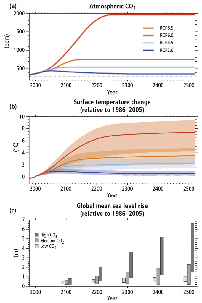
Brent Walker is right when he says that actuaries need to consider the implications of climate science in their work, but the current scientific consensus is that solar cycles are not the main driver of climate change. A better place to start in my view would be the Institute and Faculty of Actuaries report Resource constraints: sharing a finite world which points out that, either through natural depletion or the need to ration resources to mitigate climate change in the future, the primary challenge of climate change will be to manage within much stricter limits both in terms of the resources we can use and the level of economic growth we can expect. That really is something actuaries can contribute to.


When I started writing this blog in April, one of its main purposes was to highlight how poor we are at forecasting things, and suggest that our decision-making would improve if we acknowledged this fact. The best example I could find at the time to illustrate this point were the Office of Budget Responsibility (OBR) Gross Domestic Product (GDP) growth forecasts over the previous 3 years.

Eight months on it therefore feels like we have come full circle with the publication of the December 2013 OBR forecasts in conjunction with the Chancellor’s Autumn Statement. Little appears to have changed in the interim, the coloured lines on the chart below of their various forecasts now joined by the latest one all display similar shapes steadily moving to the right, advising extreme caution in framing any decision based on what the current crop of forecasts suggest.

OBR update

However, the worse the forecasts are revealed to be, the keener it seems politicians of all the three main parties are to base policy upon them. The Autumn Statement ran to 7,000 words, of which 18 were references to the OBR, with details of their forecasts taking up at least a quarter of the speech. In every area of economic policy, from economic growth to employment to government debt, it seemed that the starting point was what the OBR predicted on the subject. The Shadow Chancellor appears equally convinced that the OBR lends credibility to forecasting, pleading for Labour’s own tax and spending plans to be assessed by them in the run up to the next election.

I am a little mystified by all of this. The updated graph of the OBR’s performance since 2010 does not look any better than it did in April, the lines always go up in the future and so far they have always been wrong. If they turn out to be right (or, more likely, a bit less wrong) this time, then that does not seem to me to tell us anything much about their predictive skill. It takes great skill, as Les Dawson showed, to unerringly hit the wrong notes every time. It just takes average luck to hit them occasionally.

For another bit of crystal ball gazing in his Statement, the Chancellor abandoned the OBR to talk about state pension ages. These were going to go up to 68 by 2046. Now they are going to go up to 68 by the mid 2030s and then to 69 by the late 2040s. There will still be people alive now who were born when the state retirement age (for the “Old Age Pension” as it was then called) was 70. It looks like we are heading back in that direction again.

The State Pension Age (SPA) was introduced in 1908 as 70 years for men and women, when life expectancy at birth was below 55 for both. In 1925 it was reduced to 65, at which time life expectancy at birth had increased to 60.4 for women and 56.5 for men. In 1940, a SPA below life expectancy at birth was introduced for the first time, with women allowed to retire from age 60 despite a life expectancy of 63.5. Men, with a life expectancy of 58.2 years were still expected to continue working until they were 65. Male life expectancy at birth did not exceed SPA until 1948 (source: Human Mortality Database).

In 1995 the transition arrangements to put the SPA for women back up to 65 began, at which stage male life expectancy was 73.9 and female 79.2 years. In 2007 we all started the transition to a new SPA of 68. In 2011 this was speeded up and last week the destination was extended to 69.

SPAs

Where might it go next? If the OBR had a SPA modeller anything like their GDP modeller it would probably say up, in about another 2 years (just look again at the forecasts in the first graph to see what I mean). Ministers have hit the airwaves to say that the increasing SPA is a good news story, reflecting our increasingly long lives. And the life expectancies bear this out, with the 2011 figures showing life expectancy at birth for males at 78.8 and for females at 82.7, with all pension schemes and insurers building in further big increases to those life expectancies into their assumptions over the decades ahead.

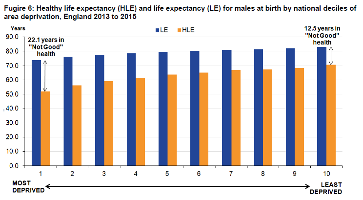
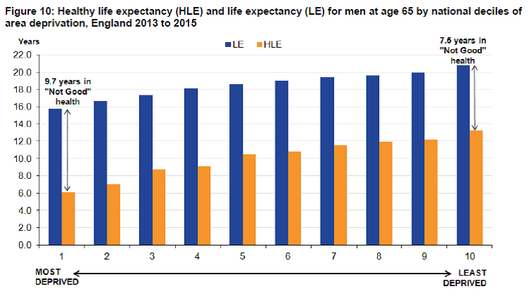
And yet. The ONS statistical bulletin in September on healthy life expectancy at birth tells a different story which is not good news at all. Healthy life expectancies for men and women (ie the maximum age at which respondents would be expected to regard themselves as in good or very good health) at birth are only 63.2 and 64.2 years respectively. If people are going to have to drag themselves to work for 5 or 6 years on average in poor health before reaching SPA under current plans, how much further do we really expect SPA to increase?

Some have questioned the one size fits all nature of SPA, suggesting regional differences be introduced. If that ever happened, would we expect to see the mobile better off becoming SPA tourists, pushing up house prices in currently unfashionable corners of the country just as they have with their second homes in Devon and Cornwall? Perhaps. I certainly find it hard to imagine any state pension system which could keep up with the constantly mutating socioeconomics of the UK’s regions.

Perhaps a better approach would be a SPA calculated by HMRC with your tax code. Or some form of ill health early retirement option might be introduced to the state pension. What seems likely to me is that the pressures on the Government to mitigate the impact of a steadily increasing SPA will become one of the key intergenerational battlegrounds in the years ahead. In the meantime, those lines on the chart are going to get harder and harder for some.

The consultation on the future shape of workplace pensions has been going on for nearly a month now and ends two weeks on Friday. It is littered with errors, from completely repeated questions (Q52 = Q54) to ones which are so similar as makes no difference (Qs 41 and 44 for example) and the thrust of a lot of the questions are quite hard to answer if you do not share some of the underlying assumptions of the DWP about the process, but come on! This is our chance to put a bit of definition into the rather blurry outline of a straw man which some of the newspapers have been tilting at so vigorously!

You don’t have to answer all of the questions, but just to goad you a bit I have done so here. Agree, disagree, I would love to hear from you. But not until you have responded to one of the following addresses:

How to respond to this consultation

Pleasesendyourconsultationresponses,preferablybye-mail,to:definedambition.pensionsconsultation@dwp.gsi.gov.uk

Or by post to:

Defined Ambition Team

Private Pensions Policy and Analysis

1st Floor, Caxton House

6-12 Tothill Street

London

SW1H 9NA


Feedback on the consultation process

There have only been 24 posts on the blog. I think the main reason for this was identified early in the process from a contributor referring to herself only as Hannah:

Hannah

I applaud the use of an open blog but it’s obvious that there’s a bit of a problem here! Perhaps, to avoid this becoming sidetracked, you could introduce a drop-down in the comment section so that people could select what aspect of DA reform or the consultation their comment relates to – and if their comment relates instead to concerns about their accrued benefits, you could redirect them to a separate specialised member queries page?

Reply

Sam Gilbert

Thanks for this Hannah, we will look into this once the blog picks up pace.

DA Team, DWP

Of course the blog never did pick up pace because people soon realised that there comments would be lost in a stream of pension benefit queries. Not the way to encourage a consultation. If you want to comment on this or anything else about the process of the consultation, the contact details are as follows:

Elias Koufou

DWP Consultation Coordinator

2nd Floor

Caxton House

Tothill Street

London

SW1H 9NA

Phone: 020 7449 7439

Email:elias.koufou@dwp.gsi.gov.uk