![]() The Government has launched a consultation into what unique arrangements could be put in place purely for the British Steel Pension Scheme (BSPS) so that:
The Government has launched a consultation into what unique arrangements could be put in place purely for the British Steel Pension Scheme (BSPS) so that:
• It won’t be a burden on the new owner of the steel business in the UK
• It won’t be a burden on the Pension Protection Fund (PPF)
• It won’t be a burden on UK PLC
The consultation document states that “In such a complex situation, the Government needs to listen to a wide range of opinions in order to decide what course of action we should take. We are therefore seeking views on the options and proposals set out in this paper. We would welcome both answers to the specific questions posed and also wider thoughts on the ideas discussed.” It therefore seems strange that they have chosen the period leading up to the EU Referendum to launch the consultation, when a wide range of opinions is likely to be the last thing they get. It is almost as if they are trying to bury a bad consultation.
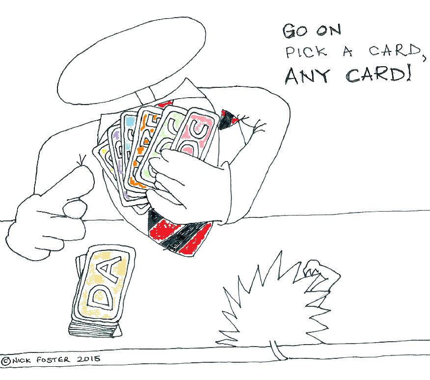
In fact it is not complicated, because this is the poor collection of options it is considering (my responses are in italics):
Option 1: Use existing regulatory mechanisms to separate the BSPS
ie the regulatory mechanisms which have been good enough for:
• MG Rover Pension Scheme
• United Industries PLC Pension Scheme – United Industries PLC section
• Caithness Glass Group Benefits Plan
• Denby 2001 Pension Scheme – DH Realisations Limited (formerly known as Denby Holdings Limited) segregated part
• Do It All Pension Plan – Do It All Ltd Section
• Allied Carpets Group Plc Pension Scheme
• Polaroid (UK) Pension Fund
• The Royal Worcester & Spode Pension Scheme
• Woolworths Group Pension Scheme – Woolworths Group Sections 129
• British Midland Airways Limited Pension and Life Assurance Scheme – UK DB Section
• Railways Pension Scheme – Relayfast Group Shared Cost Section
• Royal Doulton Pension Plan – Royal Doulton (UK) Limited segregated part of section
• HMV Group Pension Scheme
• Industry Wide Coal Staff Superannuation Scheme – UK Coal Operations Section
• Industry Wide Mineworkers Pension Scheme – UK Coal Operations Section
• The Kodak Pension Plan
• Saab GB Pension Plan – Saab Great Britain Limited segregated part
Amongst many others (only 5,945 schemes of the original 7,800 defined benefit schemes protected by the PPF remain outside).
Consultation question 1: Would existing regulatory levers be sufficient to achieve a good outcome for all concerned?
Yes. These levers were good enough for all these other schemes.
Apparently these are not good enough for Tata Steel.
Option 2: Payment of Pension Debts
Under the defined benefit pension scheme funding legislation, a sponsoring employer can chose at any time to end their relationship with the scheme – even if the scheme is in deficit. However, the employer must pay to do so.
Tata have indicated that Tata Steel UK (TSUK) would not be able to make such a payment, and that this would be unaffordable.
The usual options in this case would be:
• A sale with the pension scheme
• The insolvency of Tata Steel (how ridiculous this sounds shows that the required payment is not unaffordable)
• A sale without the pension scheme, in which case the PPF would be looking for substantial mitigation from Tata Steel and/or a share in the company in exchange for taking on BSPS
Apparently these options are not good enough for Tata Steel.
Option 3: Reduction of the Scheme’s Liabilities Through Legislation
The proposal would reduce the level of future inflation increases payable on all BSPS pensions in payment and deferment to a similar or slightly better level than that paid by the PPF. If adopted, this would mean that in the future existing pensioners would receive lower increases to their pensions than they would under the current scheme rules, or possibly no increases at all. Deferred members would also receive a lower increase to their preserved pension when they reached normal pension age, and would then receive the lower increases to their pension payments.
This approach is not without risk – which is why it is not routinely used.
Actually I am not aware it has ever been used.
Although the intention would be for the scheme to take a low risk investment strategy, there is always residual longevity and investment risk, and it is possible that the scheme would fall into deficit in the future. In the event of scheme failure, the downside risk would ultimately be covered by the PPF and its levy payers.
ie after all of the legislative hyperactivity for the benefit of one scheme, it could easily just end up in the PPF anyway.
Question 2: Is it appropriate to make modifications of this type to members’ benefits in order to improve the sustainability of a pension scheme?
No. As there is no guarantee it will improve the sustainability of the only pension scheme being considered, ie BSPS.
Regulations under section 67 of the 1995 Act
Section 67 of the 1995 Pensions Act (‘the subsisting rights provisions’) provides that scheme rules allowing schemes to make changes can only be used in a way which affects benefits which members have accrued if:
• the changes are actuarially equivalent – this means that an actuary has certified there is no reduction in overall benefit entitlement, only in the way the benefit is paid (for example, indexation is reduced but initial pension level is increased to compensate); or
• the individual member consents.
Consultation question 3: Is there a case for disapplying the section 67 subsisting rights provisions for the BSPS in order to allow the scheme to reduce indexation and revaluation if it means that most (but not all) members would receive more than PPF levels of compensation?
Ie they want to remove the need to get members’ consent before reducing their benefits. The answer is again no.
Option 4: Transfer to a New Scheme
This option would allow for bulk transfers without individual member consent to a new scheme paying lower levels of indexation and revaluation.
A bulk transfer with consent has been used previously as a mechanism for managing exceptional problems around an employer and their DB scheme.
However, the BSPS trustees have concerns about getting individual member consent to a transfer. The sheer size of the scheme means that getting member consent for a meaningful number of members would be difficult and the transfer would only be viable if enough members consented to transfer. Setting up a new scheme and transferring members to it may also need to be done rapidly in order to facilitate a solution to the wider issues surrounding TSUK – and this would be difficult to achieve in the necessary timescales if individual member consent to a transfer had to be achieved.
Consultation question 4: Is there a case for making regulatory changes to allow trustees to transfer scheme members into a new successor scheme with reduced benefit entitlement without consent, in order to ensure they would receive better than PPF level benefits?
No, as it would not ensure that they received better than PPF level benefits.
Governance of the New Scheme
The British Steel Pension Scheme (BSPS) operates as a trust. The scheme is administered by B.S. Pension Fund Trustee Limited, a corporate trustee company set up for this purpose. The assets of the Scheme are held in the name of the trustee company and, as required by law, are separate from the assets of the employers.
The trustee board has 14 members, seven are nominated by the company and seven are member-nominated trustees. The role of the trustees is to ensure that the scheme is run in accordance with the scheme’s trust deed and rules, and the pensions legal framework. The trustees’ duties are also to ensure the proper governance of the scheme and the security of members’ benefits.
Consultation question 5: How would a new scheme best be run and governed?
Under trust, separate from the assets of the employer, and subject to full existing pensions law. You could probably manage with considerably fewer than 14 trustees, but these should include member nominated trustees and, probably, a professional independent trustee.
Consultation question 6: How might the Government best ensure that any surplus is used in the best interest of the scheme’s members?
Pensions legislation already has provisions for how to apply assets to secure full benefits for members with an insurance company and deal with any surplus that occurs (it is usually set out in the scheme rules). A surplus is a highly unlikely scenario.
What the Draft Regulations Would Say
Disapplication of the subsisting rights provisions to the British Steel Pension Scheme Regulations (section 67)
These regulations would disapply the subsisting rights provisions to changes made in relation to indexation and revaluation under the BSPS Scheme Rules. This would mean that TSUK can exercise the power in the existing scheme rules to reduce levels of indexation and future revaluation to the statutory minimum without member consent. We intend to make any disapplication of the subsisting rights provisions subject to certain conditions being met to ensure member protection is not further compromised.
This is a terrible idea. Section 67 has protected many members from reductions to benefits they have already built up over the years. It should be maintained.
These would include requiring the BSPS trustees to agree unanimously that the changes to indexation and revaluation would be in the best interests of the scheme members. We are also considering whether it may be appropriate to make it a condition that the Pensions Regulator agrees to the changes being implemented.
Why has the Pensions Regulator not been asked for its view already?
Consultation question 7: What conditions need to be met to ensure that regulations achieve the objective of allowing TSUK to reduce the levels of indexation and revaluation payable on future payment of accrued pension in the BSPS without the need for member consent, balancing the need to ensure that member’s rights are not unduly compromised?
The objective is inappropriate. Disapplication of section 67 should be abandoned.
Consultation question 8: What conditions need to be met to ensure that regulations achieve the objective of allowing trustees to transfer members to a new scheme without the need for member consent, balancing the need to ensure that members’ rights are not unduly compromised.
They can’t. And this therefore shouldn’t be attempted.
All in all, a very bad consultation rushed out under cover of a much higher profile campaign.